Introduction

Picking up right where we left off in our previous blog, where we demystified the basics of linear regression and its underlying mathematics, we're now ready to take the next big step. In today's blog, we'll dive into gradient descent, a powerful optimization algorithm that plays a pivotal role in making our linear regression models even better.

What is gradient descent?

Gradient descent, at its core, is a simple algorithm in machine learning and deep learning that fine-tunes a model's parameters (m and c in linear regression case ) for the most accurate predictions.

Analogy

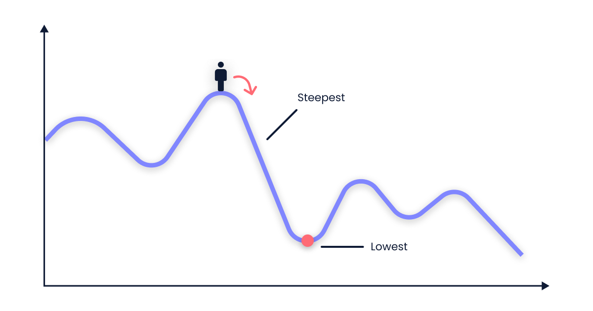
Imagine standing on a mountain peak and trying to find the quickest route to the valley below. The gradient descent algorithm works like this: at your current position, you spin around 360 degrees to find the steepest downhill direction. You then take small steps in that direction, essentially following the path of least resistance.

At each new spot, you repeat the process: spin around, locate the steepest downhill slope, and take small steps. Eventually, you'll reach the lowest point of the mountain, where the slope levels out to zero. The journey you've taken represents the set of parameters that yield the best results for your model. This easy-to-follow analogy illustrates how gradient descent optimizes parameters in the world of machine learning.

Why do we need gradient descent?

In machine learning, our primary goal is to create a model that makes accurate predictions. To achieve this, we need to optimize the model by minimizing a metric called the cost function. The cost function quantifies the error between the predicted values and the actual values, helping us evaluate the model's performance.

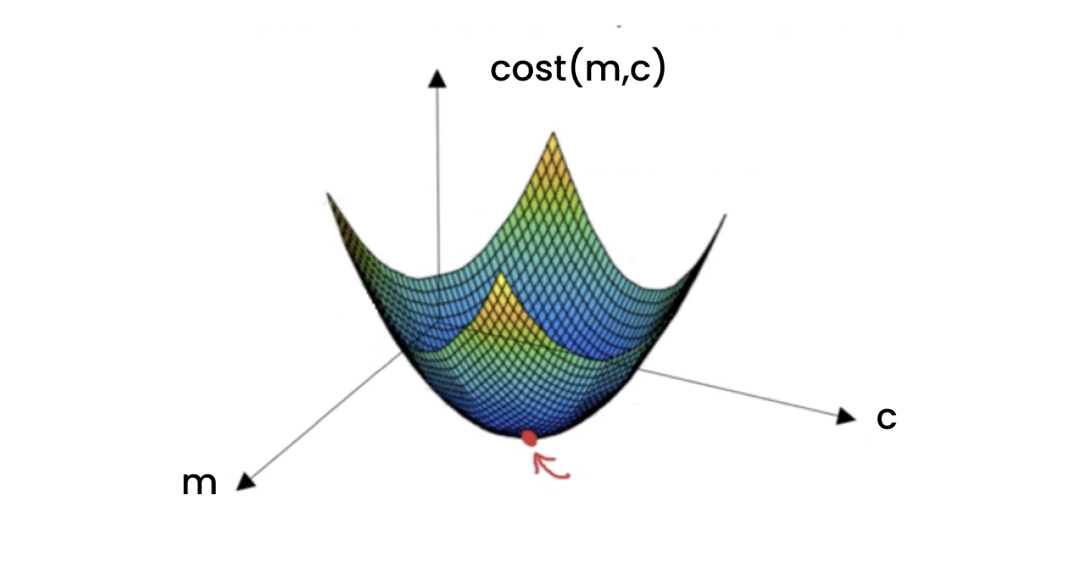
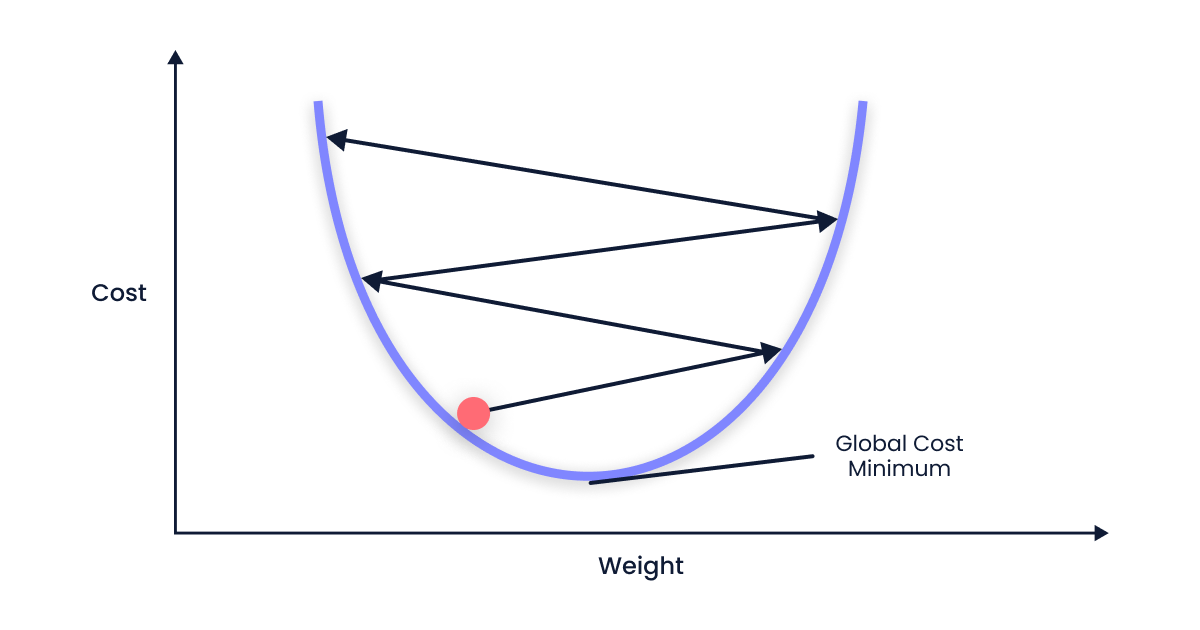
Visualize the cost function as a multi-dimensional surface with various valleys and peaks. The lowest point (global minimum) on this surface represents the optimal solution, which can be hard to locate without a systematic approach like gradient descent.

In the case of linear regression, the cost function is based on the mean squared error. This specific type of cost function results in a bowl-shaped curve as it’s a convex function, searching for the global minimum is more straightforward. Since the curve has a single lowest point, gradient descent always converges to the global minimum, resulting in an optimized linear regression model.

The formula for gradient descent

$$m_{new} = m_{old} - \alpha \frac{\partial}{\partial m}cost(m_{old}, c_{old})$$

$$c_{new} = c_{old} - \alpha \frac{\partial}{\partial c}cost(m_{old}, c_{old})$$

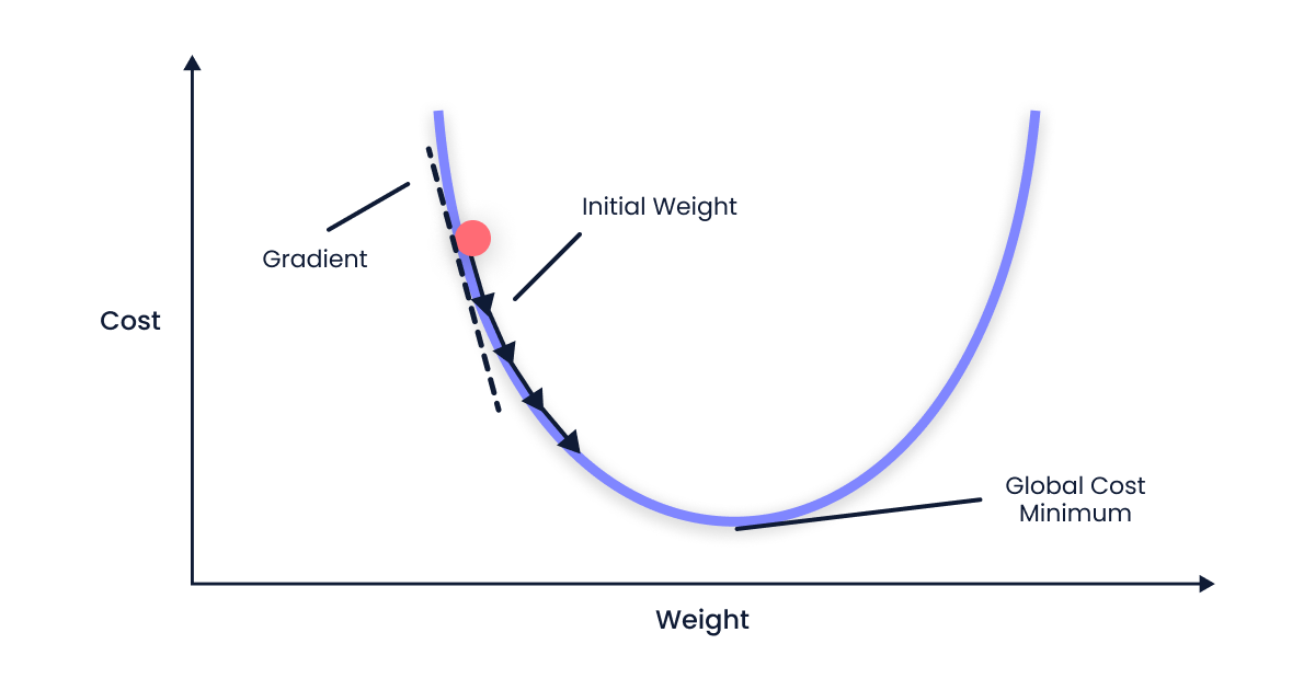
Here α is called the learning rate is a hyper-parameter it determines the step size or the rate at which the algorithm updates the model's parameters while minimizing the cost function. In essence, the learning rate controls how quickly or slowly the model converges to the optimal solution.

Gradient Descent Intuition

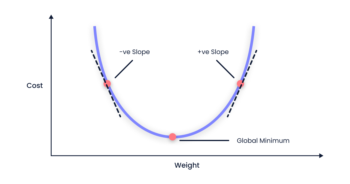
When the slope is negative

1. When the slope of the cost function (∂cost(m, c)/∂m) is negative, the weight value (m) increases because the learning rate (α) is always positive.

$$m_{new} = m_{old} + \alpha \frac{\partial}{\partial m}cost(m_{old}, c_{old})$$

1. When the slope of the cost function is negative, the value of m increases. This happens because we add a positive number to m(old). As a result, we move to the right side of the graph for our next iteration.

When the slope is positive

1. When the slope of the cost function (∂cost(m, c)/∂m) is positive, the weight value (m) decreases because the learning rate (α) is always negative.

$$m_{new} = m_{old} - \alpha \frac{\partial}{\partial m}cost(m_{old}, c_{old})$$

1. On the other hand, when the slope of the cost function is positive, the value of m decreases. This happens because we subtract a positive number from m(old). As a result, we move to the left side of the graph for our next iteration.

Learning rate (α)

Learning rate helps us to predict how big of a step we should take while finding the minimum value. The value of the learning rate ranges from 0.0 to 1.0. the learning rate that we choose might be

α is too small

When the alpha value is smaller, the steps taken in the gradient descent process will be smaller. This implies that the model's parameters will be updated more conservatively, possibly resulting in slower convergence. However, it's crucial to understand that a too-small alpha value may cause the optimization process to be too slow and take a long time to reach the global minimum, yet it can provide a better chance of not missing the smallest point.

α is too large

When the alpha value is larger, the steps taken in the gradient descent process will be bigger. This means that the model's parameters will be updated more aggressively, potentially leading to faster convergence. However, it's important to note that a too-large alpha value may cause the optimization to overshoot the global minimum and lead to divergence.

Conclusion

I hope you've enjoyed our little journey today, digging into the nitty-gritty of gradient descent and understanding its intuition. But hey, don't go anywhere just yet! We're about to turn this theory into practice in our next post. Until then, keep exploring, and happy coding!