Welcome to our comprehensive guide on Linear Regression! In this blog, my friend Hardik Nikam and I will dive deep into the world of linear regression, exploring its concept, mathematics, code implementation from scratch, and limitations. Our goal is to provide a comprehensive understanding of linear regression, so you can use it to solve real-world problems and make data-driven decisions. We've taken the time to explain everything in-depth, so even if you're new to the topic, you'll have no problem following along.

Introduction

In this guide, we will be focusing on linear regression, a specific type of supervised learning.

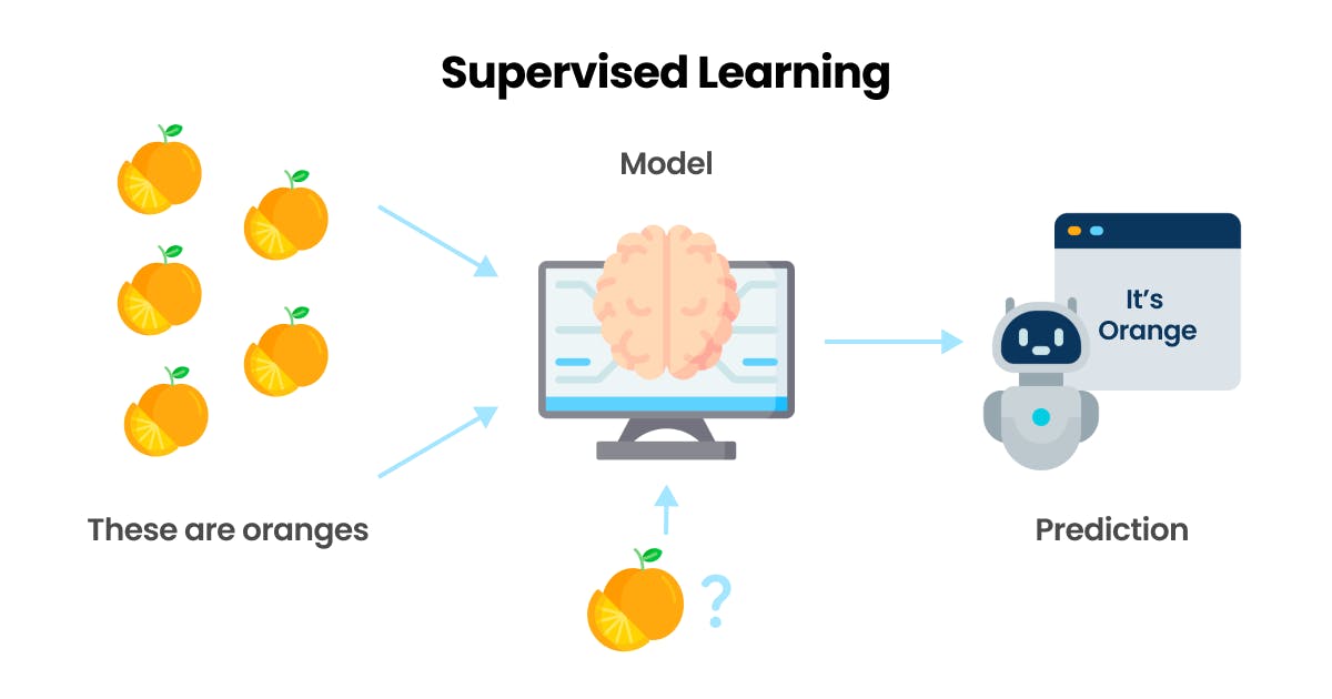
1. Supervised learning is a type of machine learning where the computer is trained using labeled data.

2. The computer is given a set of input/output pairs, and it has to learn the relationship between the inputs and outputs to make predictions on new, unseen data.

3. Linear regression is a type of supervised learning where the goal is to predict a continuous output value, like the price of a house, based on a set of input features, like the number of bedrooms or square footage.

Terminologies

When diving into linear regression, there are some key terms that you should be familiar with. Here are the most important ones:

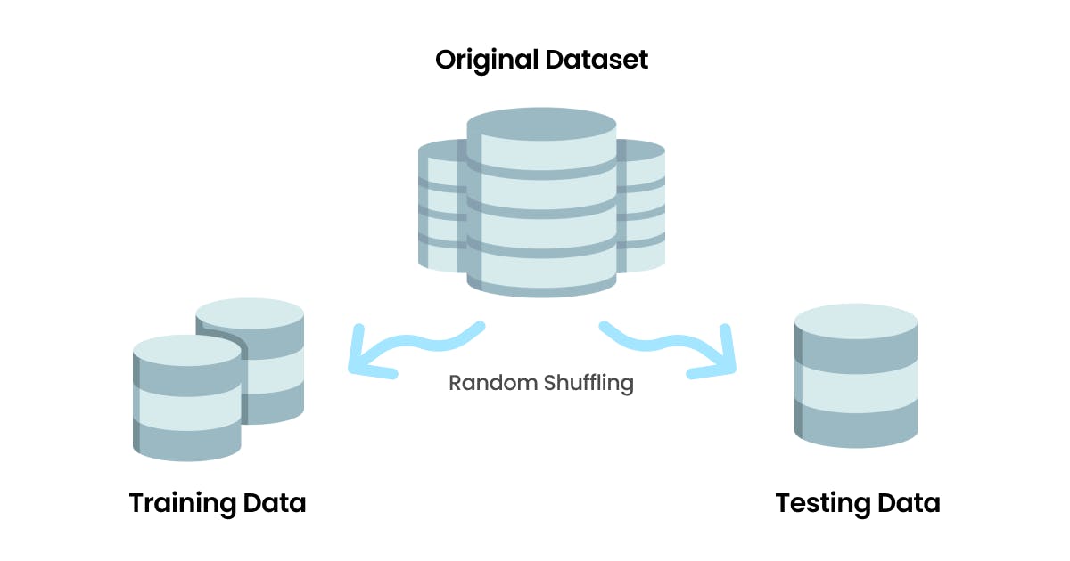
1. Training set: We partition the data set after randomization into a training set and a test set. The training set is used to train the model. The larger the training set better the model.

2. Testing set: The test set is used to test the model. It provides us with unbiased model performance with accuracy.

3. Cost function: A cost function is a mathematical function used to measure the difference between the predicted value and the actual value in the training data. Our main goal is to minimize this cost function. So the predicted value is as close to the actual value.

4. Best fit: The best fit refers to finding the line or curve that best represents the relationship between the independent variables (input) and the dependent variable (output) in the data.

5. Error: The error refers to the difference between the predicted values and the actual values. It represents how well the regression model can fit the data and make predictions.

6. Variance: The variance represents the amount by which the predictions of a model would change if different training data were used. A model with high variance tends to overfit the training data, meaning it may fit the data very well but perform poorly on new, unseen data.

7. Bias: The bias refers to the systematic error introduced by the model's oversimplification of the true relationship between the input features and output target. If a model has a high bias, it tends to make consistent predictions that are far from the true values, meaning it has poor accuracy.

How does linear regression work?

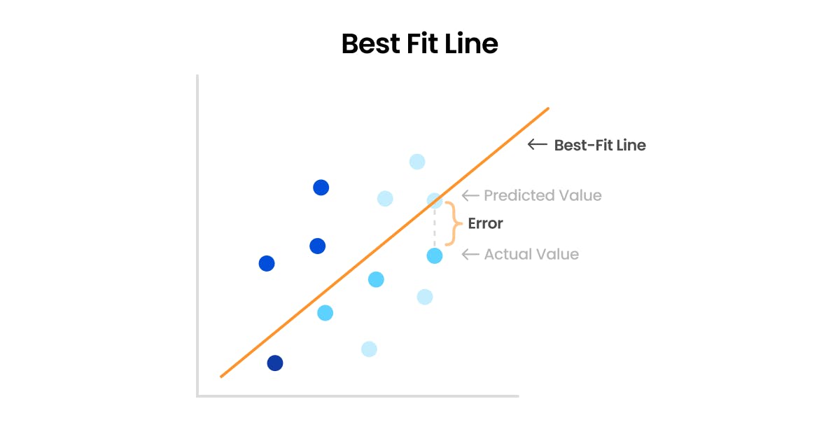
Linear regression is based on the concept of finding the best-fit line for the given data. This line should best represent the relationship between the independent variables (input) and the dependent variable (output) in the data. The objective of linear regression is to find the line that minimizes the difference between the predicted values and the actual values.

How best-fit line is derived?

The best-fit line is found using a cost function, which is a mathematical function used to measure the difference between the predicted values and the actual values in the training data. The goal is to minimize this cost function so that the predicted values are as close to the actual values as possible.

Hypothesis 1: Mean Error

The first hypothesis for a cost function is the simplest one here we sum the difference between the actual value and the predicted value.

$$\begin{equation} ME = \frac{\sum_{i=1}^n (y_a - \hat{y_p})}{n} \end{equation}$$

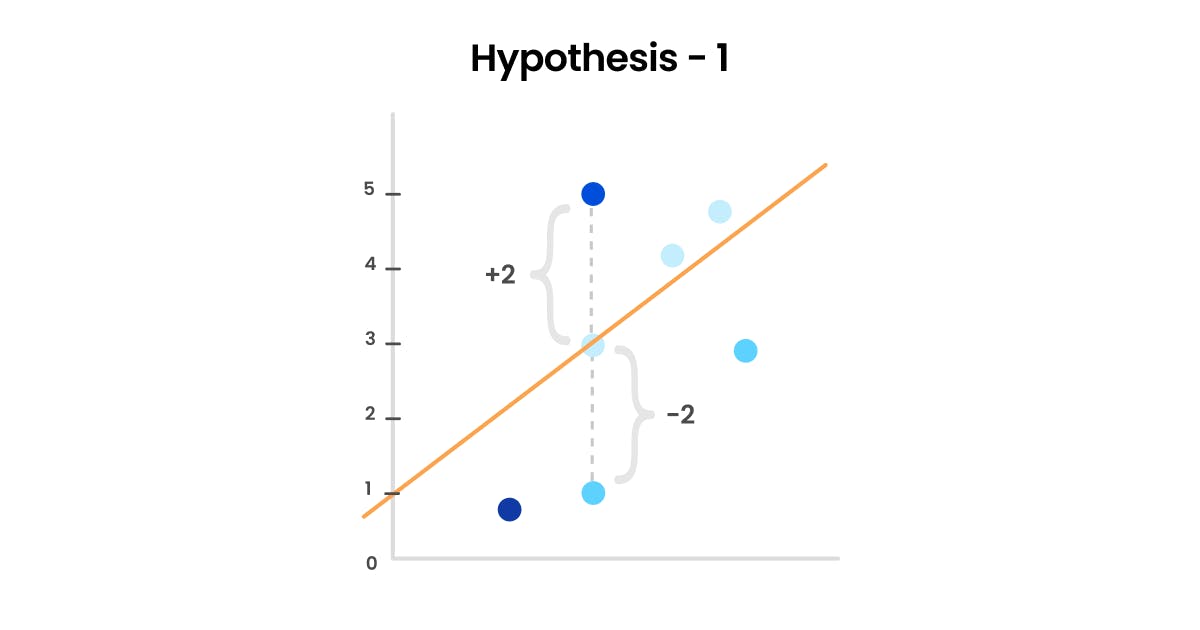
However, this approach has a major flaw. The net error can be less than the individual errors. For example, if we have an error of 2 for one prediction and an error of -2 for another, the net error would be zero, even though the actual error is 4. This is because the positive and negative errors cancel each other out. This is a clear disadvantage of using this hypothesis as the cost function, as it doesn't accurately reflect the true error.

Therefore, it's important to consider a more sophisticated cost function that takes into account the magnitude of the error, rather than just the sign.

Hypothesis 2: Mean Absolute Error

This hypothesis is an improvement over the first hypothesis as it removes the flaw of the first hypothesis where the net error could be less than the individual error. In this hypothesis, the error is calculated as the average absolute difference between the actual and predicted values. The formula for the MAE hypothesis is as follows:

$$\begin{equation} MAE = \frac{\sum_{i=1}^n |y_a - \hat{y_p}|}{n} \end{equation}$$

This hypothesis gives a more accurate representation of the actual error as it takes into account the magnitude of the error, not just its direction. The second hypothesis eliminates the disadvantage of the first hypothesis by using absolute values to calculate the error so that positive and negative errors don't cancel each other out.

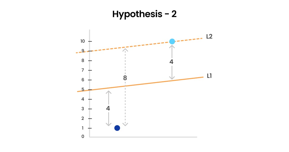
However, this hypothesis has its flaw. The second hypothesis of using absolute error has a flaw in that it punishes larger errors more than smaller errors, but it doesn't take into consideration the direction of the error. For instance, consider two best-fit lines L1 and L2. Let's say that the net error made by L1 is 8 (4, 4) and the net error made by L2 is also 8 but with an error of (8, 0). In this case, the model would consider L2 to be a better fit, even though it's trying to fit into an outlier. This is because the net error remains the same for both lines, but the absolute error for L1 is distributed evenly across the two dimensions. However, this may cause L2 to fit the data too tightly to the outliers and miss the overall trend in the data, resulting in high variance and low bias.

Hypothesis 3: Mean Squared Error

In this hypothesis, the cost function is defined as the average of the squared difference between the actual value and the predicted value. The formula for MSE is:

$$\begin{equation} MSE = \frac{1}{n} \sum_{i=1}^n (y_a - \hat{y_p})^2 \end{equation}$$

The idea behind MSE is to penalize the predictions that are far from the actual value by assigning them a higher cost. By squaring the differences between the predicted and actual values, it ensures that the errors are positive, making the cost function non-zero for any deviation from the actual value. For example, consider two best-fit lines L1 and L2. Let's say that the net error made by L1 is 8 (4, 4) and the net error made by L2 is also 8 but with an error of (8, 0). When we square these errors in the MSE formula, L1 would have an error of 32 (4^2, 4^2) and L2 would have an error of 64 (8^2, 0^2). This means that L1 is a better line to choose than L2, and the algorithm would penalize L2 more heavily. This helps the model avoid overfitting to the outliers and focus on the overall trend in the data.

MSE is a commonly used cost function for linear regression because it is differentiable and has a global minimum, making it easier to find the optimal solution using gradient descent or other optimization algorithms.

So the final formula for the cost function is:

$$\begin{equation} Cost = \frac{1}{n} \sum_{i=1}^n (y_a - \hat{y_p})^2 \end{equation}$$

$$\begin{equation} Cost = \frac{1}{n} \sum_{i=1}^n (y_a - (mx_i + c ))^2 \end{equation}$$

Tweak the cost function

As we know x is the independent variable so to minimize the cost function we need to tweak the m and c variables but how to get the value of m and c?

1. Our cost function is dependent on 2 variables(m & c)

2. We can use partial differentiation (when a function is dependent on 2 or more variables we use it.)

$$\begin{equation} \frac{\partial Cost}{\partial c} = 0 \end{equation}$$

$$\begin{equation} \frac{\partial Cost}{\partial m} = 0 \end{equation}$$

Differentiate Cost Function w.r.t "c",

$$\begin{equation} Cost = \sum_{i=1}^n (y_i - (mx_i + c ))^2 \end{equation}$$

$$\begin{equation} \frac{\partial Cost}{\partial c} = \sum_{i=1}^n \frac{\partial (y_i - (mx_i + c ))^2}{\partial c} \end{equation}$$

$$\begin{equation} \frac{\partial Cost}{\partial c} = \sum_{i=1}^n 2 \cdot (y_i - (mx_i + c )) \cdot \frac{\partial (y_i - (mx_i + c ))}{\partial c} \end{equation}$$

$$\begin{equation} \frac{\partial Cost}{\partial c} = \sum_{i=1}^n 2 \cdot (y_i - (mx_i + c )) \cdot (-1) \end{equation}$$

$$\begin{equation} \frac{\partial Cost}{\partial c} = \sum_{i=1}^n -2 \cdot (y_i - (mx_i + c )) \end{equation}$$

$$\begin{equation} \frac{\partial Cost}{\partial c} = 0 \end{equation}$$

$$\begin{equation} \sum_{i=1}^n -2 \cdot (y_i - (mx_i + c )) = 0 \end{equation}$$

$$\begin{equation} \sum_{i=1}^n (y_i - (mx_i + c )) = 0\quad...(1) \end{equation}$$

Differentiate Cost Function w.r.t "m",

$$\begin{equation} Cost = \sum_{i=1}^n (y_i - (mx_i + c ))^2 \end{equation}$$

$$\begin{equation} \frac{\partial Cost}{\partial m} = \sum_{i=1}^n \frac{\partial (y_i - (mx_i + c ))^2}{\partial m} \end{equation}$$

$$\begin{equation} \frac{\partial Cost}{\partial m} = \sum_{i=1}^n 2 \cdot (y_i - (mx_i + c )) \cdot \frac{\partial (y_i - (mx_i + c ))}{\partial m} \end{equation}$$

$$\begin{equation} \frac{\partial Cost}{\partial m} = \sum_{i=1}^n 2 \cdot (y_i - (mx_i + c )) \cdot (-x_i) \end{equation}$$

$$\begin{equation} \frac{\partial Cost}{\partial m} = 0 \end{equation}$$

$$\begin{equation} \sum_{i=1}^n 2 \cdot (y_i - (mx_i + c )) \cdot (-x_i) = 0 \end{equation}$$

$$\begin{equation} \sum_{i=1}^n (y_i - (mx_i + c )) \cdot (x_i) = 0 \quad...(2)\end{equation}$$

First, we divided both the equations by n(number of data points) as both equations are the cumulative error of all the data points we are interested in the average per data point. Then using crammers rules we solved equations 1 and 2 to get the value of m and c.

$$\begin{equation} m = \sum_{i=1}^n \frac{(x_i - \bar{x})(y_i - \bar{y})}{ (x_i - \bar{x})^2} \end{equation}$$

$$c = \bar{y} - m\bar{x}$$

where the y bar and the x bar are the mean value of x and y.

Given the values of x and y, we can use them to find the optimal values for m (slope) and c (y-intercept). These values will enable us to plot the best-fit line, which will reveal the appropriate relationship between the dependent variable (x) and the independent variable (y). By minimizing the cost function, we can determine the optimal values for m and c that will provide the line of best fit.

Conclusion

I hope this blog helped you understand the basics of linear regression, including the hypotheses, cost function derivation, and how to optimize it to get accurate predictions. We have more to cover, so stay tuned for the next blog where we'll explore optimizing the cost function using gradient descent and implementing it from scratch and with popular libraries like sklearn.